Gradient Descent: Down the Rabbit Hole
Gradient Descent: Down the Rabbit Hole
Manually doing gradient descent for regression.
Gradient descent is a method to perform mathematical optimization. You may have heard of or used gradient descent to optimize your models. In this post we will go over:
- What gradient descent is.
- Exploring a problem and a cost function
- Walkthrough of gradient descent for regression on that problem
I want to keep this post focused on the concepts; there will be code but the focus will be on getting the intuition of gradient descent.
What is gradient descent?
In machine learning most problems, classification or regression, can be represented as a process of finding some optimal function for predicting an output (target variable, label) from some set of inputs (x1, x2, x3…). One good strategy for optimization is called gradient descent.
Let’s explore a problem and a cost function
Here is some sample data from the cars data set (you can load my data here). It shows how long it takes to stop a car (dist) for cars moving at various speeds (speed). ‘dist’ is our y variable. ‘speed’ is our x variable. We will try to predict dist from speed.
import pandas as pd
# load the data
data = pd.read_csv('cars.csv')
data.head()
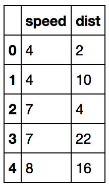
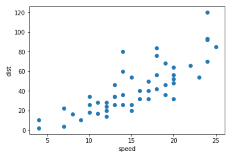
Our data looks like this, and we want to draw a line through it that is optimized to fit the data as closely as possible:
plt.scatter(data['speed'], data['dist'])
plt.xlabel('speed')
plt.ylabel('dist')
plt.show()
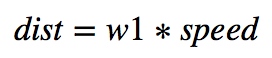
We will make a function with one parameter (w1):
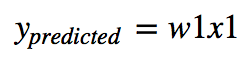
We will evaluate this model with a cost formula for a single w1:
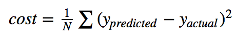
We subtract the actual speed from our predictions of speed, square the difference, and average over all examples. The lower a cost value is the better. If we calculate this cost out for many values of w1 we get a ‘cost function.’ This cost function shows different costs for differnet values of w1.
Let’s plug in some data and lets try some w1 values to see what our cost function looks like:
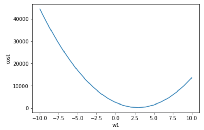
Practically speaking we should exepect a positive value for w1 as a higher speed should require a longer stopping distance. It looks like the lowest cost value of this regression is around w1=2.6 (right above 2.5). So y=2.6x1 is the optimal function for predicting the stopping distance from speed for the cars dataset. So that’s it everyone! This post is over; let’s call it a day!
So…it’s actually more complicated than that. Here the cost function can be calculated because our ‘problem space’ (the number of possible combinations of possible parameter and input values) is small. We only have one parameter (w1) and one input (x1). If our prediction function was more complicated (more parameters and more inputs) it would take a long time to compute the actual shape of its cost function and to find the lowest cost. For linear regression calculating the cost function has an O(n³) computation time, where n is the number of features/inputs. With 20 parameters it takes 8000 times longer (20³) to calculate the cost function than for 1 parameter. Most problems in the real world are complicated and are usually represented with many parameters and so have expensive to compute cost functions.
Enter Gradient Descent
So if it is too expensive to compute the cost function for real world problems how do we find the optimal function? Gradient descent is the process of following a ‘gradient’ downwards to reach the lowest cost. It is a way to solve for the parameter that produces the lowest cost without computing the whole cost function. How can you compute a gradient?
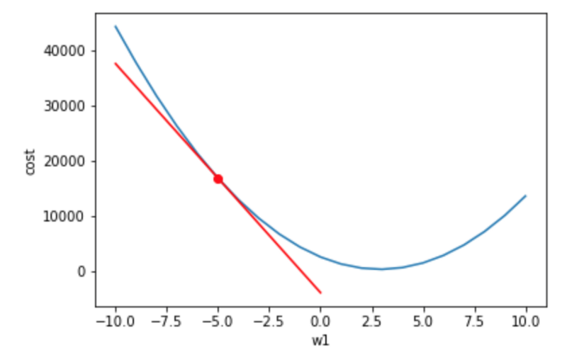
Draw a tangent line from the current point; get the slope of that line (code):
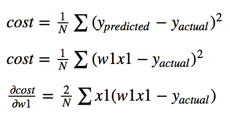
Compute the derivative and plug in the current point (use the chain rule to calculate the partial derivative of cost wrt. w1):
Once you get the gradient you can subtract it from your current prameter value to move down the cost function. Basically you are calculating the slope towards the lowest cost and then moving you parameter value (w1) in that direction. But you may notice the tangent line above is a bad approximation if you move far enough away from the original point. If you move too far along the tangent line you get the wrong value for w1 and a 0 cost (not actually possible). This is why you just take a ‘small step’ along the direction of the gradient using something called a learning rate. Here the learning rate is 0.001. It keeps you close to your original point and stops you from getting a bad w1. Here we have repeated the gradient dsecent process 15 times (frames =15).
Starting at w1= -10 and animated the process of fitting the best regression line looks like so (see code):
Starting at w1 = -10 and animated this process of finding the lowest cost looks like so (see code):
Notice our gradient becomes 0 and settles on the lowest possible cost value. Also notice how the changes in w1 become smaller near the end as we get close to our optimal value. The lowest cost value ends up being at w1=2.9. So our original estimate of about 2.6 was not too bad. Hopefully you have a more intuitive undestanding of how gradient descent works now!
Quick tips:
- Stick to well known loss functions. Early on in this post I tried to simplify the loss function to make this post easier to understand, it turns out this can create complications that cause gradient descent to move away from an optimal point (aka the exploding gradient problem).
- Make sure to use a differentiable loss function. If you are using a custom loss function check its differentiability manually or with wolfram alpha. Your loss function should have a computable derivative. If your loss function is not differentiable you can’t use gradient descent.
- Brush up on your calculus, specifically chain rule/partial derivatives. Read “Calculus Made Easy” if you don’t know calculus. It will help you to prove/derive things for yourself when you need to understand what your code is doing. Calculus is the single most useful tool I learned in school. We probably could have skipped the rest of the ‘curriculum.’
I hope you enjoyed this post of gradient descent. If you want to signup for my newsletter covering marchine learning for video games and see more datascience you can do that here. Have a good day!