Jun 2018
CLPR 3D Cubes
Today I’m releasing the cLPR dataset, a dataset for doing work in 3D machine learning. The name stands for Cubes for Learning Pose and Rotation. The goal is to provide a nice baseline dataset of colored 3D cubes in many different positions for testing machine learning algorithms whose goal is to learn about pose and rotation.
Download the dataset here:
The Data
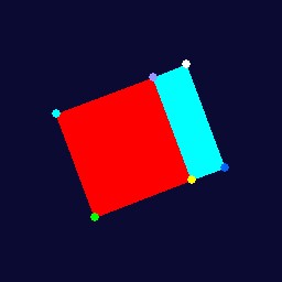
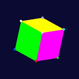
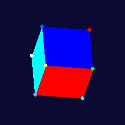
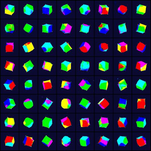
The dataset contains 32x32, 64x64, 128x128, 256x256 jpeg images of a cube (2d projections of the 3d object). The jpegs do not have any quality loss. The data looks like this:
The Labels
The labels are provided in the binary numpy file. The file is called cube1–1.14.3–2018–06–10–12–30–10.npy, generally cubeN-x.xx.x-datetime.npy where x.xx.x is the numpy version used to dump the file and N is the cube this data file is for. It contains every position and rotation of the nodes in a cube for all images in the dataset. For this dataset the structure is 250047 x 8 x 6, It’s POSITIONS x NODES x 6 numpy array, where the first 3 values of the last dimension (0,1,2) are x,y,z position and the last 3 values in the last dimension (3,4,5) are x,y,z rotation in radians. You can also create whatever labels you want by modifying the script stores in the rotation_positions array (projector.py, line 90). So the structure looks like:
Making the Dataset
The dataset is produced using a package called pygame, a package originally designed for making python games. The package is nice because it lets you easily draw and render objects in 2d or 3d. I used pygame because I wanted the code to be easy enough for someone with limited graphics experience and basic knowledge of matrix multiplication to understand.
Step 1 Create a Wireframe
First we create a wireframe of the cube. This wireframe consists of nodes, edges, and faces. The nodes are points in space, each represented with x,y,z coordinates. We store all the nodes in an 8x3 numpy array. Edges are two nodes (the indices of the nodes in the numpy array). Faces are 4 nodes connected (the indices of the nodes in the numpy array). You can create a wireframe like this:
I use this to create 8 nodes, 6 faces. You don’t need to specify edges, just nodes and faces. You can test a cube wireframe creation; run python wireframe.py script included in the repository:
For this wireframe class, the only outside dependency for wireframe.py is numpy. This script will create a cube and print the nodes, edges, and faces.
Step 2 Generate Rotations
Then I generate a set of rotations I’d like to apply in 3D to the nodes of the cube (the corners of the cube). I loop through all possible combinations of rotations from 0-6.3 radians(close to 2π radians but not exactly perfect) to generate the rotations.
The above snippet will generate roughly 360 degrees, 2π of rotation in radians. Then every frame/iteration of pygame, we will grab one of these rotations and display it.
Step 3 Render the Wireframe
I render the wireframe using pygame’s functions to draw polygons. The function takes a series of edges (2 points, [(x,y,z), (x,y,z)]) and draws a polygon on-screen with that color in the order of the points and edges given. Below is a quick and dirty version of my code; the actual script is more involved.
Step 4 Apply one Rotation and Re-Center the Cube
To apply a rotation to this cube, I use a rotation matrix for the appropriate axis. So to rotate around the x-axis, I would use create_rot_x from wireframe.py. This function returns a matrix for doing rotations in the x-axis for the number of radians we need. Then I do a dot product in the transform function between the nodes of the wireframe and the rotation matrix we created. All this does is multiply the x,y,z positions of our nodes by the right numbers in the matrix such that the new positions are rotated by however many radians along x. I repeat the above process for x,y and z radians for this rotation. After this is done, re-center the cube, so its middle is around the center of the screen.
Step 5 Reset the cube nodes to their initial position
I store the initial position and reset it to that after every rotation+re-center+snapshot of the cube. This makes it easier to reason about what the cube does on every iteration and move to exactly the rotation I give it. Unfortunately, moving from one rotation to another can also have problems with something called gimbal lock. It is a bit of a mind-bender, so I wanted to avoid it entirely.
Step 6 Repeat Steps 3–5
While I do this, I screenshot the pygame screen after every rotation and store position information in a numpy array. During the process, I write the images to disk, and at the end, I save a numpy array with all the nodes’ positions and rotations.
Final step: Visual inspection and programatic testing of labels
I playback the numpy file (the -t input option to projector.py does playback of npy file) and watch the rotations that look good. Also, run it through the test_npy_positions function (the -n input to projector.py), which compares it against known correct values for the positions at every section. The explanations above are intended to give you a sense of how the code works. See the code on github for more details. The code is not perfect, neither is the dataset, and there’s a lot of room to improve (i.e., adding color mappings to the labels to make tracking easier). Please feel free to make a pull request or hack around on your own. I would appreciate it.
What can you do with this dataset?
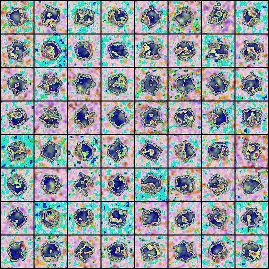
One thing you can do is train variational autoencoders. To show an example of how to use this dataset I’ve provided two variational autoencoders (one classic, one convolutional). Both are a bit underwhelming, underwhelming but the point is to show an example, not to have a perfect model. Below is a picture where each cell represents an area of the latent space I have sampled and then put through our decoder network to generate a cube:
Not all of these look like cubes, but hey, a couple of them do! The code is in this notebook. Generative models are notoriously finicky. Here’s an example of one of my failed model outputs:
Here is the obligatory gif (snapshot at every epoch) of the vae model I made above training on a subsample of the data:

If you would like a much better example of autoencoders trying different distributions in the autoencoder please check out this paper (and accompanying github code), written by my friend Tim Davidson at Universiteit van Amsterdam and several of his colleagues. There is also a cool paper on SO3 autoencoders using a variant of this dataset.
Conclusion
Thanks for making it to the end. If you find an issue with the dataset or any of the scripts, please reach out to me; people are already using this data (pre-release) for research papers and projects, so issues should be known, publicized, and debugged. If you would like to cite this dataset you can do so:
@misc Scher:2018,
author = "Yvan Scher",
year = "2018",
title = "cLPR Dataset",
url = "https://bit.ly/2yeeA15",
institution = "The Internet"
If you enjoyed this post, be sure to signup for more.